Design Lessons from Biomorphs
I really have been led to think differently as a result of creating, and using, computer models of artificial life which, on the face of it, owe more to the imagination than to real biology. The use of artificial life, not as a formal model of real life but as a generator of insight in our understanding of real life, is one that I want to illustrate in this chapter. (Dawkins 1989, p239)
In “The Blind Watchmaker”, Richard Dawkins introduced a simple computer model to illustrate the power of incremental cumulative change. His model mapped a compact digital genome to a branching graphical form. These forms, which Dawkins dubbed Biomorphs, took on a wide range of natural forms and abstract shapes (see Dawkins 1986, p61).
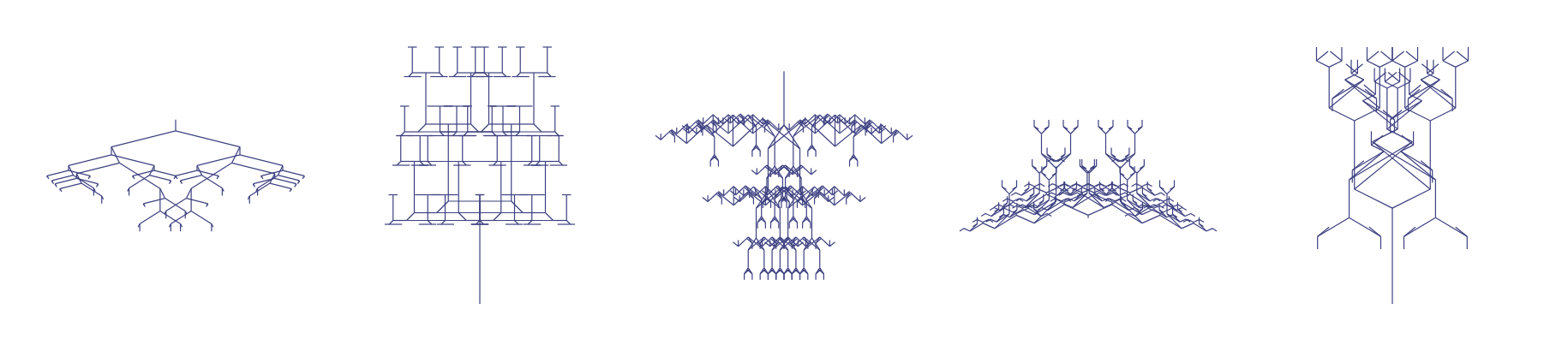
Figure 1 displays a menagerie of these Biomorphs, each generated from Dawkins’ original algorithm: a mantis, a cocktail bar, a carousel, a crab, and a bear rug.
The visual appeal of the Biomorphs comes from a simple but cleverly designed algorithm. I’ll use this algorithm as a starting point to think highlight some key factors about designing a model of development and evolution.
Building a Biomorph
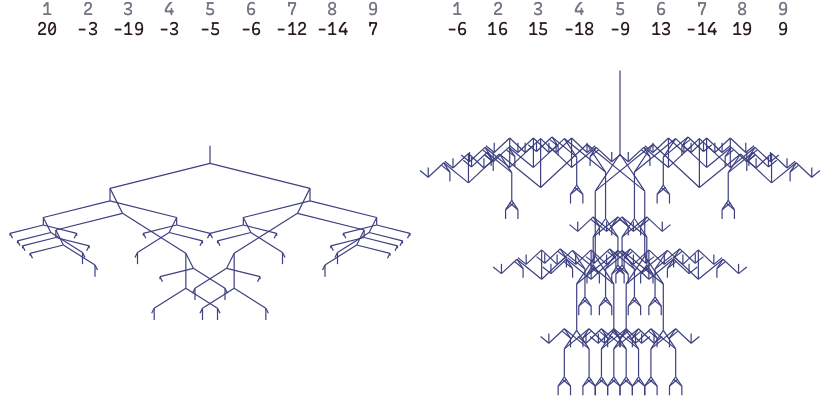
Every Biomorph begins with a genome: an array of nine integers that control how the form will grow. Figure 2 shows two Biomorphs—the mantis head and carousel—with their genomes displayed above them.
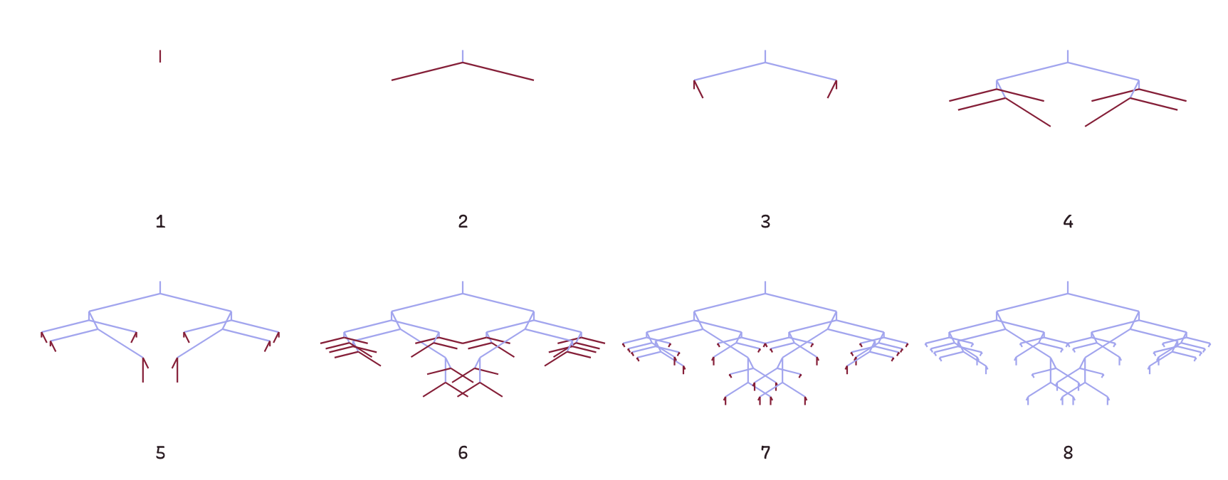
To produce a Biomorph, the drawing algorithm uses the genome as a set of parameters. The algorithm by growing tree, starting with a single vertical trunk (see frame 1 in Figure 2). At the tip of each branch, it faces the same choice: stop growing, or sprout two new branches. The ninth gene determines how many times the biomorph will branch before stopping. You can see the carousel Biomorph is far bushier than the mantis head because it has nine, rather than seven levels of branching.
When the Biomorph does continue growing, it must determine which direction the new branches should point—and this is where the other eight genes come in.
The eight directional genes work in pairs. Each pair specifies horizontal and vertical offsets for the end of the next branch from the current branching point. Let’s say the two genes were 5 and 2. The end of the next branch would be 5 steps up from the current position. And, depending on whether the branch is on the left or right, it would go left 2 steps or right 2 steps. This last constraint ensures the Biomorphs have bilateral symmetry.
As the algorithm grows the tree, it cycles through these four pairs of genes, reusing the same directional instructions at each level. In addition, branch lengths shrink with each generation. You can see the effect of re-using the same genes with shorter branch lengths in Figure 3. The branches in the 6th frame point in the same directions as those in the 4th frame, they are just shorter. This gives the Biomorphs a distinctive, fractal-like appearance.1
Walking in Biomorph Space
The power of the Biomorph system lies in how mutations translate to form. Since the genome consists of integers, a mutation simply adds or subtracts small values from these numbers.2 The algorithm’s design ensures that these small genetic changes produce correspondingly small changes in shape. This makes it possible to connect two radically different Biomorphs by a chain of tiny mutations.
Consider the transformation from carousel to mantis head shown in Figure 4. We create this lineage by interpolating between the two genomes, generating a series of intermediate forms. Each step represents a single small mutation, yet the cumulative effect is dramatic. The carousel’s circular symmetry gradually distorts and stretches until the mantis emerges.3
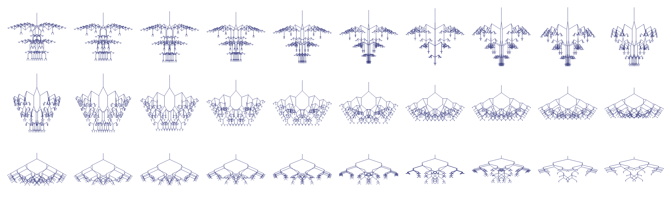
This chain demonstrates precisely what Dawkins wanted to show: incremental changes in genes (nine integers) can accumulate to produce dramatic differences in phenotype (the visual form).
Surprise: No Populations, No Selection
Nothing in my biologist’s intuition, nothing in my 20 years’ experience of programming computers, and nothing in my wildest dreams, prepared me for what actually emerged on the screen (Dawkins 1986, p59).
Dawkins designed the algorithm to produce Biomorphs. Yet the output still astonished him. This is not unusual; it reflects a common experience with computational models where simple rules often generate unexpectedly rich behavior. But the source of his surprise reveals something important about evolutionary modeling.
For some wonderful examples of simple models generating complex behaviour, see Conway’s Game of Life, the fractal structure of the logistic map, and Reynolds’ Boids.
The Blind Watchmaker aimed to solve what Dawkins called “the greatest of all mysteries” (Dawkins 1986, pxiii): how apparent functional design arises in nature without a designer. The book’s central argument championed Darwin’s theory of evolution by natural selection as the answer. Given this focus, you might expect Dawkins’ amazement to stem from witnessing the power of natural selection that he built into his model.
Yet here’s the twist: the Biomorph model contains no populations, no fitness measurements, and no selection algorithm at all. Dawkins did employ artificial selection, using his aesthetic preferences to guide exploration through Biomorph space. But the key point here is that selection of any kind—artificial or natural—can only navigate the landscape that the underlying algorithm creates.
What truly surprised Dawkins was not the power of selection but the extraordinary richness of the Biomorph space itself. This richness emerged entirely from his choices in designing the genotype-phenotype mapping. Dawkins himself recognized this point in his later work on evolvability:
The type of embryology that we choose for our artificial life is crucial. This is another way of stating the key message of this chapter (Dawkins 1989, p239).
This insight doesn’t displace the role of natural selection for solving the puzzle of apparent design in nature. The Biomorph-drawing algorithm determines what forms are possible, but exploring this vast space without a guiding hand requires some automated process. Darwinian selection provides one powerful approach to this exploration.
But the fact remains that when building models capable of generating surprising or novel outcomes, the selection algorithm rarely poses the greatest challenge. The critical design decision—the one that determines whether your model will produce rich, unexpected behavior—lies in crafting the genotype-phenotype mapping. Design a mapping right, and even random exploration can surprise you.
This insight extends beyond computational models to our understanding of biological evolution itself. This was recognised in one of the most influential early papers on evolvability, by Wagner and Altenberg (Wagner and Altenberg 1996). Wagner and Altenberg recognised that the experience of building computational models to produce complex adaptations highlighted just how important the genotype-phenotype mapping was. And they emphasized how biologists might miss this crucial aspect when studying evolution, as they are already studying the outcomes rather than the processes that generate them.
The process of adaptation can proceed only to the extent that favorable mutations occur, and this depends on how genetic variation maps onto phenotypic variation. […] Biologists are not confronted by this problem because they study the end products of evolution, which are prima facie evidence that the favorable mutations have occurred at a sufficient rate. (Wagner and Altenberg 1996)
Designing a Genotype-Phenotype Space
[…] before any Darwinian process can get going, there has to be a bare minimum of conditions set up. These were the conditions that I had to engineer in my computer world (Dawkins 1989, p239)
The transformation sequence in Figure 4 represents a journey through genotype-phenotype space—the set of all possible pairings between genetic codes and the forms they produce. Thus far, I’ve focused largely on the mapping from genotype to phenotype. But creating such a space requires more than this. So what are the essential components?
Dawkins captured these requirements in a diagram that I’ve adapted in Figure 5.4 His framework reveals the minimal architecture needed for any evolutionary system.

Dawkins titled his diagram “Weismann’s continuity of the germ plasm (expressed in Pascal).” This refers to August Weismann’s 19th-century insight about the separation of hereditary information from body cells. It also references Pascal, the programming language Dawkins used for his implementation. While the Biomorphs represent one specific realisation, this same architecture underlies virtually all computational evolutionary models.
Weissman was a German evolutionary biologist who proposed the Weismann barrier, which states that hereditary information passes only from germ cells (egg and sperm) and not from somatic (body) cells.
The architecture consists of four components—two processes and two data structures:
- Genotype. A compact, structured representation that persists and varies across generations. In biology, this corresponds to DNA or the genome. In Biomorphs, it’s the array of nine integers.
- Phenotype. The observable outcome produced when the mapping function processes the genotype. Biological phenotypes encompass all physical and functional traits—shape, color, behavior. The Biomorph phenotype is the visual pattern drawn by the algorithm.
- Mapping function. Dawkins labels this DEVELOPMENT. This process transforms genotype into phenotype. While the Biomorph version operates deterministically, more sophisticated mappings might incorporate noise, environmental inputs, or adaptive responses.
- Mutation operator. Dawkins calls this REPRODUCTION. This transformation generates variant genotypes from existing ones. In Biomorphs, it simply perturbs numeric values. More complex systems might include recombination, mutational biases, or structural constraints. Crucially, the mutation operator defines the notion of distance in genotype space.
These four elements suffice to construct a genotype-phenotype space. They form the foundation for thinking about designing a minimal epigenesis. Note that we still haven’t introduced selection—that comes later, operating over the space these components create. The critical design decisions center largely on the mapping function and, secondarily, on the mutation operator.
Where to Next?
Dawkins’ Biomorphs endure as an elegant demonstration of genotype-phenotype space design. Decades on, the variety of forms that emerge from nine simple numbers remains striking. Despite their simplicity, they led to insights about evolvability, that how development is organised governs what evolution can readily find.
If nine integers can do this, what might richer mappings reveal?
References
Calcott, Brett. 2009. “Lineage Explanations: Explaining How Biological Mechanisms Change.” British Journal for the Philosophy of Science 60 (1): 51–78.
Dawkins, Richard. 1986. The Blind Watchmaker. New York : Norton.
———. 1989. “The Evolution of Evolvability.” In Artificial Life. Routledge.
Wagner, Gunter P., and Lee Altenberg. 1996. “Complex Adaptations and the Evolution of Evolvability.” Evolution 50 (3): 967–76. https://doi.org/10.2307/2410639.
Footnotes
For more detail on how the biomorph algorithm works, see chapter 3 of Dawkins (1986). For an overview of the technical details, see Dawkins (1989).↩︎
In practice, we also limit the range of these integers, to prevent bifurcations from being too few or numerous, and to ensure branches are neither too long nor too short.↩︎
The idea of reconstructing a lineage of related forms, showing the incremental changes required to transform one form into another is I have a called Lineage Explanations (Calcott 2009). Importantly, these explanations require neither populations, nor selection.↩︎
I changed the orientation of the diagrams. Evolutionary time is horizontal, and Development is vertical. I also removed the terms of the Pascal programming language terms that Dawkins used. The original diagram is in Dawkins (1986), p240.↩︎